In my previous post, I showed that MetrixLT can multiply two hourly data series even though the software was not designed for that specific purpose.
Finding unintended uses of MetrixLT proved to be an addicting game for our forecasting staff.
Naturally, the next question is: “If we can multiply, can we divide?”
Since division is multiplication with an inverse, we thought this might be easy. But once again, MetrixLT was not designed for performing simple arithmetic, and creating the inverse still requires dividing.
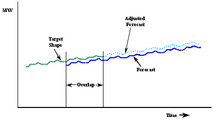
The MetrixLT Scaling Transformation is designed for two functions. First, The Scaling Transform can be used to adjust a forecast based on the historic ratio between the backcast and a Target series. If I have a forecast of hourly load for 2018 and a backcast covering 2017 (defined as the Overlap), then I can adjust the forecast based on the ratio of the Target series to the Overlap. While interesting, this is not the designed operation we will use for division.
To divide, we will use the second Scaling Transformation function designed to calibrate a bottom-up forecast to a Target series. Assume you have a Target series Y and three bottom-up series A, B, and C. The Scaling Transform can adjust A, B, and C such that Y= A+B+C. The process is two-fold. First, the Scaling Transform calculates the Calibration series (kCalib) as shown below.
kCalib = Y/(A+B+C).
Second, the Scaling Transform applies the Calibration series to each of the bottom-up series.
A’ = A x kCalib
B’ = B x kCalib
C’ = C x kCalib
The division process takes place in calculating kCalib. To divide interval data, we must make Y one series and the bottom up components (A, B, and C) and single a different series (D). The resulting ratio is the division outcome.
kCalib = Y/D.
Division can be accomplished using the following steps.
Step 1: Import Interval Data
Import the hourly data in the Interval Data table. In this example, hourly data for Zone 1 and Zone 2 are imported. I’ve highlighted the January 11, 2015 values to check our work.
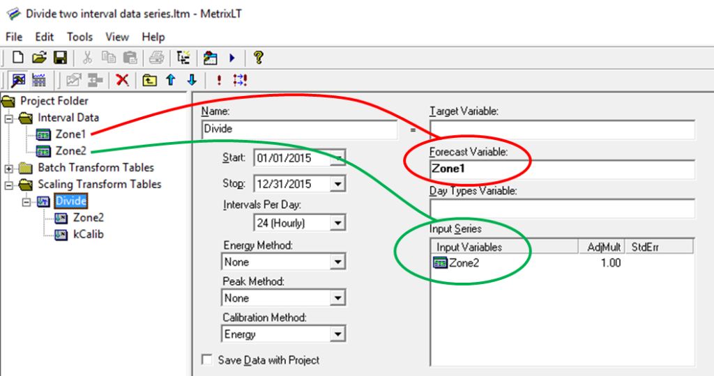
Step 2: Configure A Scaling Transformation
Create a Scaling Transformation and configure the Forecast Variable and the Input Series boxes. In the Forecast Variable box, insert the hourly data used as the numerator. In the Input Series box insert the hourly data used as the denominator. In the example, Zone1 is the numerator and Zone 2 is the denominator.
When the Target Variable is undefined, the Energy Method, Peak Method and Calibration Method selections do not apply.
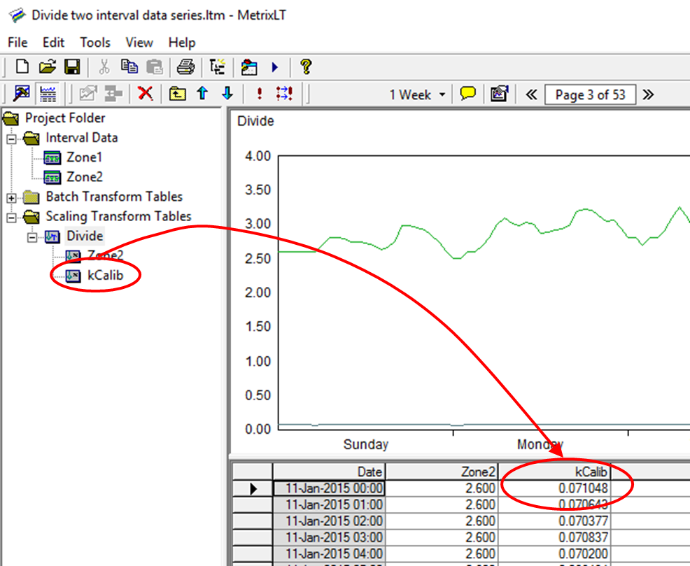
Step 3: Calculate the Result
Select the “!” to calculate the Scaling Transformation. The division result is stored in the kCalib variable.
I’ve highlighted the validation for January 11, 2015.
Zone 1 = 2.60
Zone 2 = 36.595
Product = (Zone 1) / (Zone 2) = 0.071048
Zone 1 values are divided by Zone 2 values and stored in a kCalib variable of the Scaling Transformation table.
Mark Quan is a Principal Forecast Consultant with Itron’s Forecasting Division. Since joining Itron in 1997, Quan has specialized in both short-term and long-term energy forecasting solutions as well as load research projects. Quan has developed and implemented several automated forecasting systems to predict next day system demand, load profiles, and retail consumption for companies throughout the United States and Canada. Short-term forecasting solutions include systems for the Midwest Independent System Operator (MISO) and the California Independent System Operator (CAISO). Long-term forecasting solutions include developing and supporting the long-term forecasts of sales and customers for clients such as Dairyland Power and Omaha Public Power District. These forecasts include end-use information and demand-side management impacts in an econometric framework. Finally, Quan has been involved in implementing Load Research systems such as at Snohomish PUD. Prior to joining Itron, Quan worked in the gas, electric, and corporate functions at Pacific Gas and Electric Company (PG&E), where he was involved in industry restructuring, electric planning, and natural gas planning. Quan received an M.S. in Operations Research from Stanford University and a B.S. in Applied Mathematics from the University of California at Los Angeles.