Behind-The-Meter Solar Generation and Real-Time Load Forecasting – Part 3
April 26, 2017
Share this story on:
In my blog posting “Behind-The-Meter Solar Generation and Real-Time Load Forecasting,” I presented four load forecasting challenges that have arisen as the result of deep penetration of behind-the-meter (BTM) distributed energy resources (e.g. solar generation), time-of-use rates, demand response programs, BTM storage, and electric vehicle charging. These four challenges are:
Challenge 1. Growing Disconnect between Measured Load and Demand for Electricity Services
Challenge 2. The Relationship between Measured Load and Weather is Becoming Cloudy
Challenge 3. Increased Load Forecast Errors and Error Volatility
From a load forecasting perspective, these challenges are leading to an evolution in the way we develop models and forecasts. In my second blog on this topic, I introduced the steps that Itron is taking to address the first three challenges. In this blog, I introduce an approach for constructing load forecast confidence bounds that leverages a modeling technique applied widely in financial markets.
Why do we need confidence bounds? From the perspective of scheduling and dispatching generation, the confidence bounds provide valuable input to the decisions around how much generation should be held in reserve in case observed load conditions deviate from forecasted load conditions. The concept of spinning reserves addresses the operational reality that the unexpected is expected. But holding excess generation in reserve comes at a cost. In the ideal world, these costs would be minimized if the unexpected could be accurately forecasted. As load forecasters, we may not be able to forecast all the unexpected events that could occur (e.g. drivers taking out transformers, squirrels jumping upon sagging transmission lines), but we can quantify the load forecast uncertainty.
What are the sources of load forecast uncertainty? First, the very loads that the load forecast models are built on are subject to measurement error. In many cases, what a system operator sees as load is a result of detailed calculation rather than the aggregate sum of metered demand. Specifically, load is computed as Total Generation + Net Imports - Transmission and Distribution Losses. In some systems, this calculation is straightforward and results in a solid estimate of load. In other systems, the network topology is complex and forming a clean definition of what points are “in” the system versus what points are part of another system is subject to redefinition. You might be surprised by the number of times we have been called in to fix a model only to discover that the load forecast deviations were due to a redefinition of load that was driven by the addition of a new transmission line to the network topology.
Second, with deep penetration of BTM solar generation what we measure as load is a proxy for the demand for electricity services. Because BTM solar generation is volatile, this volatility is translated to an increased volatility of measured load. This in turn increases load forecast uncertainty because the target we are trying to hit is bouncing around more frequently and in growing amplitude.
The third source of load forecast uncertainty is weather forecast uncertainty. This will not come as a surprise to anyone that makes a living based on vagaries of weather forecasts. Weather forecast error comes in a couple flavors. First, most weather forecasts under forecast hot temperatures and over forecast cold temperatures. Essentially, most weather forecasts tend to ride in between the two extremes. Some of this is a result of a weather vendor taking a weighted average of several high level model forecasts, where the high level model forecasts reflect different weather scenarios. The process of averaging pulls the point forecast away from the extremes and toward the center of the weather scenarios. Second, because weather forecasts are a derivative of a model there arises the possibility that the forecasts have a systematic model bias at certain times of a day. For example, I have seen the case where the weather forecast was consistently 2 degrees warmer at 6am and 7am regardless of the rest of the weather forecast. This consistent over forecast is a derivative of the weather forecast model. Finally, there are catastrophic weather forecast error which is when all the high level weather models simply get it wrong by 5 degrees (F) or more. Another flavor of a catastrophic weather forecast error is missing the timing of a weather front as it moves through a service territory. Catastrophic weather forecast error is the hardest to control for, but unfortunately these are the days that are remembered by management because those are the days the load forecast was way wrong.
The final source of load forecast uncertainty is the load forecast framework which includes both the load forecast models and any manual interventions that are applied to the model forecasts. Despite what people think, statistical models are subject to error. Simply put, there are too many things that drive the demand for electrical services to model individually. The art of load forecast model development is to capture systematic load patterns with the goal that what is left unexplained has the signature of random noise. Large well behaved systems are easier to model because the law of large numbers works in our favor. The random, non-systematic behavior of millions of households and businesses when aggregated together tends to smooth out to repeatable and predictable load patterns. In these cases, what is left unexplained tends to be random noise. Further, that noise as a percentage of total load tends to be less than 0.50%. When load forecast models are fitted to smaller systems or to loads with more granular geographic specificity the law of large numbers breaks down. As a result, the ratio of noise to repeatable load patterns goes up. This, in turn leads to greater load forecast uncertainty.
What makes good confidence bounds? Good confidence bounds should quantify the load forecast uncertainty with respect to each source of load forecast uncertainty. Further, good confidence bounds should be sensitive to the forecast horizon. For example, if the forecast horizon is five minutes from now and we are utilizing a highly autoregressive model, the main source of load forecast error will be measurement error rather than temperature forecast error. In contrast if the forecast horizon is day-ahead then the temperature forecast error grows in importance. Intuitively, we expect the confidence bounds to widen the further into the forecast horizon, resulting in what would look like cone shape bounds. We also expect that the confidence bounds would be time-of-day, day-of-the-week, and potentially season dependent.
Together, this suggests taking a modeling approach to developing the confidence bounds. It turns out that Dr. Robert F. Engle who won a Nobel Prize in Economics for his seminal paper "Autoregressive Conditional Heteroscedasticity with Estimates of the Variance of United Kingdom Inflation". Econometrica. 50 (4): 987–1008. 1982 describes a modeling approach that we can leverage to forecast the desired load forecast error variances. Dr. Engle’s Autoregressive Conditional Heteroscedasticity (ARCH) model can be written generically as follows:
This may not look like anything special, but what if we construct the by taking the sequence of hour-ahead load forecast errors and squaring them. Now, I can set up a simple regression model of the hour-ahead forecast error variance as:
Here, we have a one period autoregressive model where the current hour ahead load forecast error variance is a function of the prior hour, hour ahead load forecast error variance. Of course, we could extend the autoregressive terms by including the prior two, three, four, five, …, up to k hour values of the hour ahead load forecast error variances. This is the AR part of ARCH.
The Conditional Heteroscedasticity (CH) part of ARCH can contain explanatory variables that would allow the forecast error variance to vary by the time-of-day, day-of-the-week, season and potentially the weather forecast. To illustrate, let me build out an ARCH model for the one-hour ahead load forecast error variance for the load forecasts made at 7am for 8am. The ARCH model could look like the following:
Like any regression model, the specification of the ARCH model is wide open. With some experimentation, the right set of autoregressive and heteroscedastic terms can be decided upon. The result will be a model that can be used to forecast the load forecast error variance for the one hour ahead forecast of 8am loads that was made at 7am. In practice, this means there will be 24, load forecast error variance models for each forecast horizon (say 1 hour ahead through to 24 hours ahead).
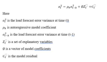
To incorporate Weather Forecast Uncertainty, we can extend the model as follows:
Here, we added the estimated Weather Forecast Error Variance as another explanatory variable in the model. In this particular case, the Weather Forecast Error Variance would be based on the one-hour weather forecast errors. The Weather Forecast Error Variance itself would be derived from a second ARCH model of weather forecast error variances.
In a similar fashion, we could extend the ARCH model to include forecasts of BTM solar generation and the associated BTM solar generation forecast error variance. An example would be as follows:
As you can see, there are no limits to the variables that you can include in the ARCH model. The ARCH framework provides a general framework for forecasting load forecast error variances that allow us to go beyond simple +/- two model standard errors to functions of forecasted weather and solar generation.
The challenge we face is deciding on the right set of explanatory variables to include in our ARCH models. This is where experimentation is required. I recommend starting with the heteroscedastic pieces: day-of-the-week, season, weather, BTM solar, predicted weather error variances, and predicted BTM solar error variances. Once you have found a set of explanatory variables that explain the heteroscedastic error variance, you can start layer in the autoregressive terms.
With the deep penetration of BTM solar generation, battery storage, and other distributed energy resources, what is measured as load is no longer a perfect measure of the demand for electricity services. In my first blog, I identified a list of load forecasting challenges that result from this erosion of measuring the demand for electricity services. From a load forecasting perspective, these challenges are leading to an evolution in the way we develop models and forecasts. In my second blog, I presented solutions for improving short-term load forecast performance. In this third blog, I introduce a general modeling framework for constructing load forecast confidence bounds that incorporates weather and BTM solar generation forecast uncertainty.
I want to leave you with one final thought. The salient operating feature of the new distributed energy resources (i.e. Solar PV and Other Generation, Storage, TOU Pricing, and Demand Response) is their variability. If all these technologies worked on pre-defined or predictable operating schedules, the forecasting challenge would be similar to incorporating long-run trends in energy efficient appliances which lower loads, but do not add load variability. It is the added load variability that comes with the new distributed energy resources that is causing the erosion in load forecast performance. As a result, the load forecast modeling problem extends beyond capturing average load swings to include capturing the volatility around the average loads. Put simply, it is no longer sufficient to forecast the mean, but we need to also forecast the variance. I believe, in time, the forecast of the load variance will be more important from a system operations point of view than the point forecasts operators get today. This may seem like a small step, but like most things in life, big things come from small steps. “That’s one small step for man, one giant leap for mankind”, Neil Armstrong circa 20 July, 1969.
Dr. Frank A. Monforte is Director of Forecasting Solutions at Itron, where he is an internationally recognized authority in the areas of real-time load and generation forecasting, retail portfolio forecasting, and long-term energy forecasting. Dr. Monforte’s real-time forecasting expertise includes authoring the load forecasting models used to support real-time system operations for the North American system operators, the California ISO, the New York ISO, the Midwest ISO, ERCOT, the IESO, and the Australian system operators AEMO and Western Power. Recent efforts include authoring embedded solar, solar plant, and wind farm generation forecast models used to support real-time operations at the California ISO. Dr. Monforte founded the annual ISO/TSO Forecasting Summit that brings together ISO/TSO forecasters from around the world to discuss forecasting challenges unique to their organizations. He directs the implementation of Itron’s Retail Forecasting System, including efforts for energy retailers operating in the United Kingdom, Netherlands, France, Belgium, Italy, Australia, and the U.S. These systems produce energy forecasts for retail portfolios of interval metered and non-interval metered customers. The forecast models he has developed support forecasting of power, gas and heat demand and forecasting of wind, solar, landfill gas, and mine gas generation. Dr. Monforte presides over the annual Itron European Energy Forecasting Group meeting that brings together European Energy Forecasters for an open exchange of ideas and solutions. Dr. Monforte directed the development of Itron’s Statistically Adjusted End-Use Forecasting model and supporting data. He founded the Energy Forecasting Group, which directs primary research in the area of long-run end-use forecasting. Recent efforts include designing economic indices that provide long-run forecast stability during periods of economic uncertainty. Email Frank at frank.monforte@itron.com, or click here to connect on LinkedIn.